Archive for Technical

Time series

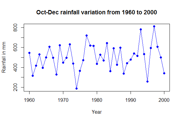
Interannual variation of OND rainfall

Data: download

#Read data
b.data <- read.table(“timeseries.csv”, header=T,fill=T)
# Scatterplot Matrices from the glus Package
attach(mtcars)
#library(gclus)
library(scatterplot3d)
attach(b.data)
# TIMESERIES1
plot(Rainfall~Year, cex = 1, col = “blue”, type=”o”, pch=19, ylab=”Rainfall in mm”, main = “Oct-Dec rainfall variation from 1960 to 2000”)
timeseries

Scatterplot 2D

Data:download

R Script
par(mar=c(5,6,4,3)+0.1) # set marigin
b.data <- read.table(“3dscatterogram.csv”, header=T,fill=T) # read input data
attach(b.data)
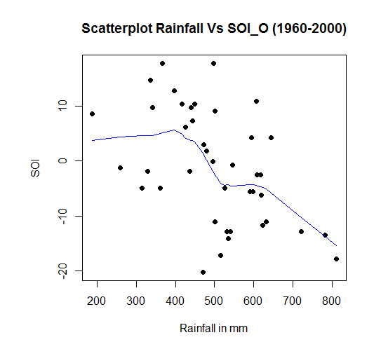
plot(Rainfall, SOI_O, main=”Scatterplot Rainfall Vs SOI_O (1960-2000)”, xlab=”Rainfall in mm”, ylab=”SOI”, pch=19) # plot function
# Fit planes
abline(lm(Rainfall~SOI_O), col=”red”) # regression line (y~x)
lines(lowess(Rainfall,SOI_O), col=”blue”) # lowess line (x,y)

2dScatterograma

Scatterogram 3D

Data: download

#Read input data
b.data <- read.table(“3dscatterogram.csv”, header=T,fill=T)
# call scatterplot3d package
library(scatterplot3d)
attach(b.data)
# simple 3d scatterplot
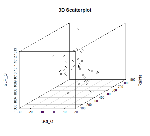
scatterplot3d(SOI_O,Rainfall,SLP_O, main=”3D Scatterplot”)

scatterogram3da

# 3d scatterplot with Fit planes
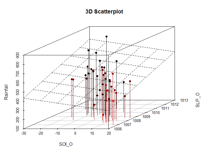
s3d <-scatterplot3d(SOI_O,SLP_O,Rainfall, pch=16, highlight.3d=TRUE, type=”h”, main=”3D Scatterplot”)
fit <- lm(Rainfall ~ SOI_O+SLP_O)
s3d$plane3d(fit)

scatterogram3db

Scatterogram matrix

Data: Download

R Script

b.data <- read.table(“scatterogram.csv”, header=T,fill=T)
# Scatterplot Matrices from the glus Package
library(gclus) # call gclus package
dta <- b.data[c(5,4,3,2)] # get data
dta.r <- abs(cor(dta)) # get correlations
dta.col <- dmat.color(dta.r) # get colors
# reorder variables so those with highest correlation
# are closest to the diagonal
dta.o <- order.single(dta.r)
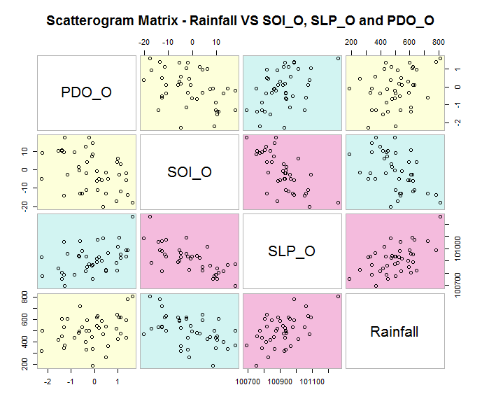
cpairs(dta, dta.o, panel.colors=dta.col, gap=.5,
main=”Scatterogram Matrix – Rainfall VS SOI_O, SLP_O and PDO_O” ) # plot title

scatterogram

Box plots

Data: Download

R Script

#Read input data
b.data <- read.table(“boxplot.csv”, header=T,fill=T)
# Plot boxplot in single color
#boxplot(b.data,ylab =”Rainfall in mm”, las = 2, at =c(1,2,3,4,5), names = c(“Trichy”,”Cuddalore”,”Mettur”,”Naga”,”Salem”))

boxplot1

# Plot boxplot in multi color

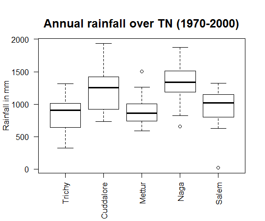
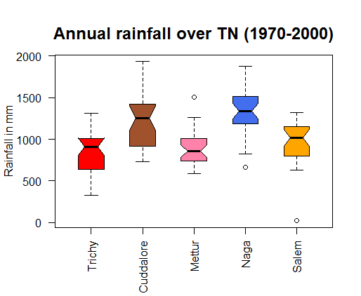
boxplot(b.data,ylab =”Rainfall in mm”, col = c(“red”,”sienna”,”palevioletred1″,”royalblue2″,”orange”),las = 2, at =c(1,2,3,4,5), names = c(“Trichy”,”Cuddalore”,”Mettur”,”Naga”,”Salem”),boxwex = 0.5, notch = T)

boxplot2

# Add headings to the plot
mtext(“Annual rainfall over TN (1970-2000)”, side = 3, line = 1, cex = 1.5, font = 2)


QQ Plots

QQ PLOTS & Regression line

Data: download

#Set margin
par(mar=c(5,6,4,2)+0.1)
b.data <- read.table(“qqplot.csv”, header=T,fill=T)
library(car)
fit <- lm(Cuddalore~Nagapattinam, data=b.data)
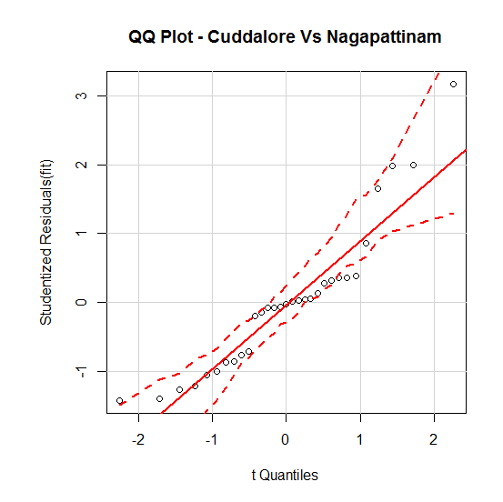
qqPlot(fit, main=”QQ Plot – Cuddalore Vs Nagapattinam”)

qqplot